The idea of boosting is to generate a committee learner $f(x)$ by aggregating many weak learners $f_m(x)$. A weak learner should generate estimates better than a trivial prediction rule (such as a constant regression function or random labeling) by exploiting some information from the feature(s). However, we do not require a weak learner to fit an arbitrary regression function or Bayes classifier.

Here, we discuss two common choices of weak learners.

Stumps #

Suppose we have a univariate feature $X\in\mathbb{R}$ for a target $Y\in\mathcal{Y}\subset\mathbb{R}$. An example of weak learner is the stump that assigns different constant outputs in two regions $\{x\in\mathcal{X}: x<\theta\}$ and $\{x\in\mathcal{X}: x>\theta\}$

$$g(x;\theta,c_1,c_2)=\begin{cases}c_1& x<\theta\\c_2 & x> \theta\end{cases}.$$ We omit the boundary case $x=\theta$ for simplicity. In practice, one can often adjust the threshold (slightly) to avoid boundary issues; otherwise we can assign any of the possible labels.

The threshold $\theta\in\mathbb{R}$ and the constants $c_1,c_2\in\mathcal{Y}$ are parameters that should be fitted. We should keep $c_1\neq c_2$; if a constant prediction is needed, one could set $\theta$ small enough instead.

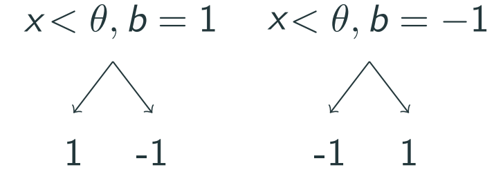
For the two-class classification problem with $\mathcal{Y}=\{-1,1\}$, there are only two possible combinations of outputs: $$(c_1,c_2)\in\{(-1,1),(1,-1)\},$$ corresponding to what-we-called decision stumps given by $$g(x;\theta,b)=\begin{cases}b& x<\theta\\-b & x> \theta\end{cases},\quad b=\pm 1.$$ Collecting the set of decision stumps yields a small space of candidate prediction rules: $$\mathcal{G}=\{g(x)=\operatorname{sign}(\theta-x)\cdot b: \theta\in\mathbb{R},~ b=\pm 1\}.$$ which can be illusrated as follows:

The left node shows the output when the condition $x<\theta$ is true, and the right node shows the output when the condition is false.

For a multivariate input vector $$x=(x_1,\ldots,x_d)\in\mathbb{R}^d,$$ we allow the user to choose one of features to split on. The set of decision stumps is then given by $$\begin{align*}\mathcal{G}=\{g(x)&=\operatorname{sign}(\theta-x_j)\cdot b:\\\ &j\in\{1,\ldots,d\}, \theta\in\mathbb{R},~ b=\pm 1\}.\end{align*}$$

$\Tau$-terminal node Tree #

A $\Tau$-terminal node tree is a prediction rule $g$ that partitions the domain set $\mathcal{X}$ into possibly more disjoint region $\{\mathcal{R}_{\tau}:\tau=1,\ldots,\Tau\}$ and output the prediction $g(x)=c_{\tau}$ if $x\in \mathcal{R}_{\tau}$. We can represent it using the additive form given by $$\begin{align*}&g(x;\{c_{\tau},\mathcal{R}_{\tau}:\tau=1,\ldots,\Tau\})\\&=\sum_{\tau=1}^{\Tau}c_{\tau}\mathbf{1}(x\in \mathcal{R}_{\tau}).\end{align*}$$ It is easy to verify that any stump splitting on the $j$-th feature is a 2-terminal node tree with $$\mathcal{R}_{1}=\{x\in\mathcal{X}: x_j<\theta\}\\\mathcal{R}_{2}=\{x\in\mathcal{X}: x_j>\theta\}.$$

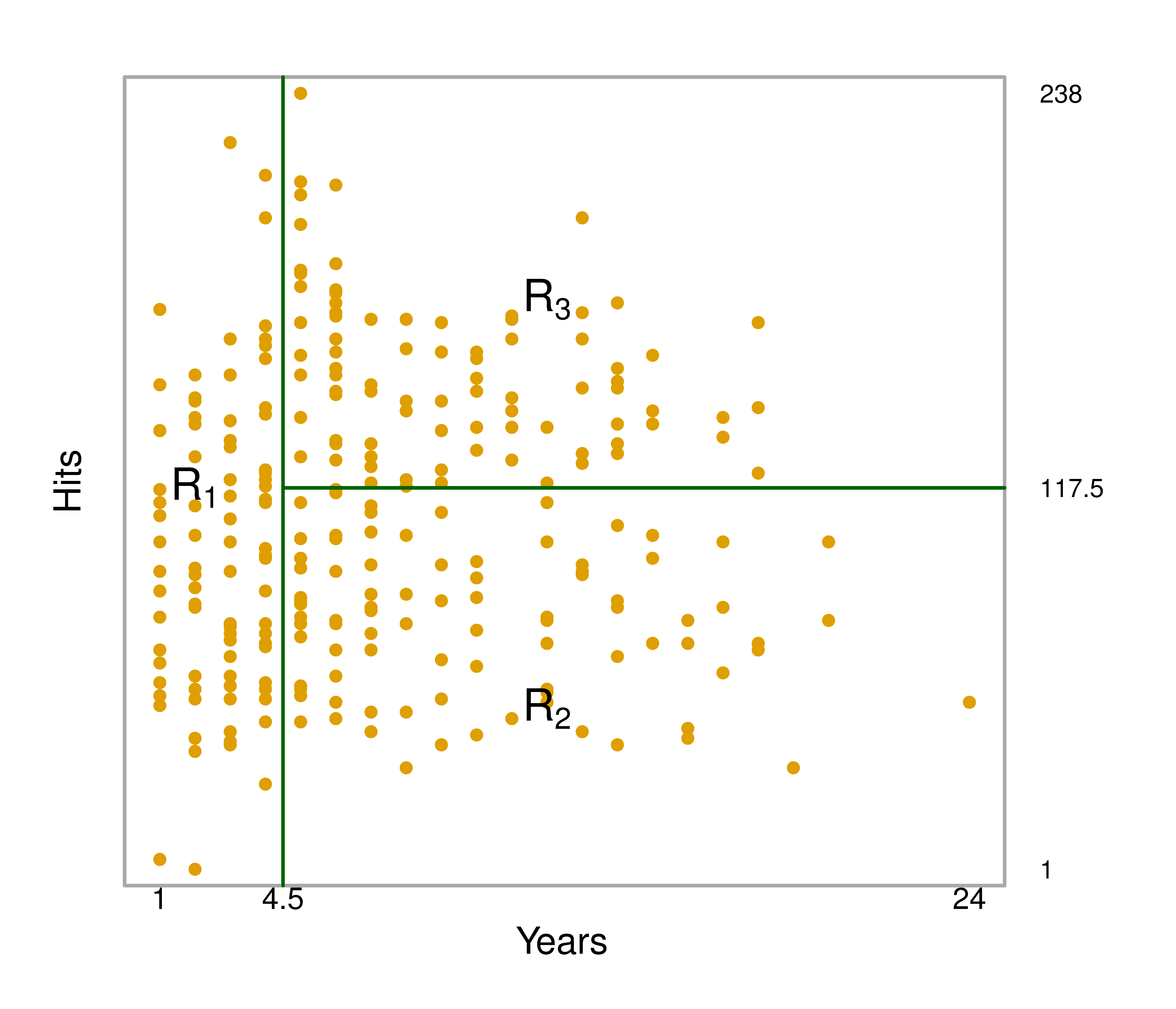
The parameters of this base learner are the coefficients $\{c_{\tau}\}$, and the quantities that define the boundaries of the regions $\{\mathcal{R}_{\tau}\}$. The common practice to consider only rectangular regions and below is an illusration of a partition with $\Tau=3$ regions for the ‘Hitters’ data from James et al. (2021):

The variable on the x-axis is the number of years that the male baseball player has played in the major leagues, whereas the variable on the $y$-axis is the number of hits he made in the previous year.

A good choice could be $\Tau=11$, for example, if one wants to use a small tree but relatively larger than a stump.

Span of Base Class #

Let $\mathcal{G}$ be a base class of weak learners, particularly stumps, such that $g\in\mathcal{G}$ if and only if $-g\in\mathcal{G}$. The span of the base $\mathcal{G}$, denoted by $\operatorname{span}(\mathcal{G})$, is the collection of the weighted sum $$f(x)=\sum_{m=1}^{M}\alpha_mg_m(x),\quad \alpha_m\geq 0,~ g_m\in\mathcal{G}$$

over all possible choices of $M\in\{1,2,\ldots\}$. Note that each $\alpha_m$ is a constant that does not depend on $x$, while each $g_m(x)$ is a function of $x$. If we define $f_m(x)=\alpha_mg_m(x)$, we can simplify the additive form into a unweighted version given by $$f(x)=\sum_{m=1}^{M}f_m(x),\quad f_m\in\mathcal{B},$$ where $$\mathcal{B}=\{f(x)=\alpha g(x): \alpha\geq 0, g\in\mathcal{G}\}.$$ For stumps $g(x)\in\mathbb{R}$ allowing for any real-valued outputs, it is easy to show that $\mathcal{B}=\mathcal{G}$. On the contrary, for decision stumps with binary output $g(x)\in\{-1,1\}$, $\mathcal{B}\neq \mathcal{G}$. However, here it is always true that $\operatorname{span}(\mathcal{B})=\operatorname{span}(\mathcal{G})$.

The goal of boosting algorithms is to find an ideal prediction rule $f\in \operatorname{span}(\mathcal{G})$, or equivalently $f\in \operatorname{span}(\mathcal{B})$, that (nearly) minimizes some risk function.