Consider the structural equations again but allowing the potential outcomes to be non-linear in confounders such that $$Y_i=\delta D_i+ \mu^{(0)}(X_i)+\varepsilon_i,$$ where $\mu^{(0)}$ is the regression function for the control group given by $$\mu^{(0)}(x)=\mathbb{E}[Y_i^{(0)}|X=x].$$

Learning Bias #

Suppose that we have a machine learning estimator $\widehat{\mu}^{(0)}$ from an auxiliary sample (e.g., from another country) independent of our observations such that $$\mathbb{E}b(X_i)=0$$ but with a nonzero conditional bias given by $$b(x)=\mathbb{E}[\widehat{\mu}^{(0)}(x)]-\mu^{(0)}(x)\neq 0,~x\in\mathcal{X}.$$ This estimation bias typically emerges due to the bias-variance tradeoff nature in the regularization procedures.

Now rewrite the regression model to be $$Y_i-\widehat{\mu}^{(0)}(X_i)=\delta D_i+\widetilde{\varepsilon}_i$$ with the new errors $$\widetilde{\varepsilon}_i=\varepsilon_i-\eta_i(X_i)-b(X_i),$$ where $\eta(x)=\widehat{\mu}^{(0)}(x)-\mathbb{E}\widehat{\mu}^{(0)}(x)$.

The conventional least-squares estimator of $\delta$ is then given by $$\begin{align*}\widehat{\delta}=&\left(\sum D_i^2\right)^{-1}\sum D_i(Y_i-\widehat{\mu}^{(0)}(X_i))\\=&\delta+\left(\sum D_i^2\right)^{-1}\sum D_i\widetilde{\varepsilon}_i.\end{align*}$$

However, the error term may suffer from an estimation bias if $$\mathbb{E}[D_i \widetilde{\varepsilon}_i]=-\mathbb{E}[D_ib(X_i)]\neq 0.$$ as the confounders $X_i$ can influence both $D_i$ and $b(X_i)$. This issue is understood as endogeneity in econometrics.

Debiased Machine Learning #

In the spirit of double selection, one may eliminate the learning bias by exploiting the structural equation for the treatment assignment dummy:

$$D_i=p(X_i)+v_i,~\mathbb{E}[v_i|X_i]=0.$$

If the error $v_i$ were observable, one can use it as a valid instrument for $D_i$ as

$$\mathbb{E}[v_iD_i]=\mathbb{E}v_i^2\neq 0$$ but using the law of iterated expectations $$\begin{align*}&\mathbb{E}[v_i\widetilde{\varepsilon}_i]\\=&\mathbb{E}[v_i\varepsilon_i]-\mathbb{E}[v_i\eta(X_i)]-\mathbb{E}[v_ib(X_i)]\\=&0-\mathbb{E}[\underbrace{\mathbb{E}[v_i|X_i]}_{0}\cdot \eta(X_i)]\\&-\mathbb{E}[\underbrace{\mathbb{E}[v_i|X_i]}_{0}\cdot b(X_i)]=0.\end{align*}$$ Hence, $$\delta=\frac{\mathbb{E}[v_i(Y_i-\widehat{\mu}^{(0)}(X_i)]}{\mathbb{E}[v_iD_i]}.$$ Replacing the expectations with their sample analogies gives an asymptotically unbiased estimator of $\delta$.

In reality, however, the errors $v_i$ are unobservable. One should use the auxiliary sample (independent of our observations) to construct an estimator $\widehat{p}(x)$ of the conditional propensity score functions $p(x)$. Then we can estimate the errors $v_i$ by $$\widehat{v}_i=D_i-\widehat{p}(X_i)$$ and then the estimator of $\delta$ is given by $$\widehat{\delta}=\left(\sum_{i=1}^{n} \widehat{v}_iD_i\right)^{-1}\sum_{i=1}^{n} \widehat{v}_i (Y_i-\widehat{\mu}^{(0)}(x_i)).$$

If an auxiliary sample is unavailable ad hoc, we typically split the data into two independent folds and use one fold as the auxiliary sample for the other fold. This method is called double machine learning or debiased machine learning.

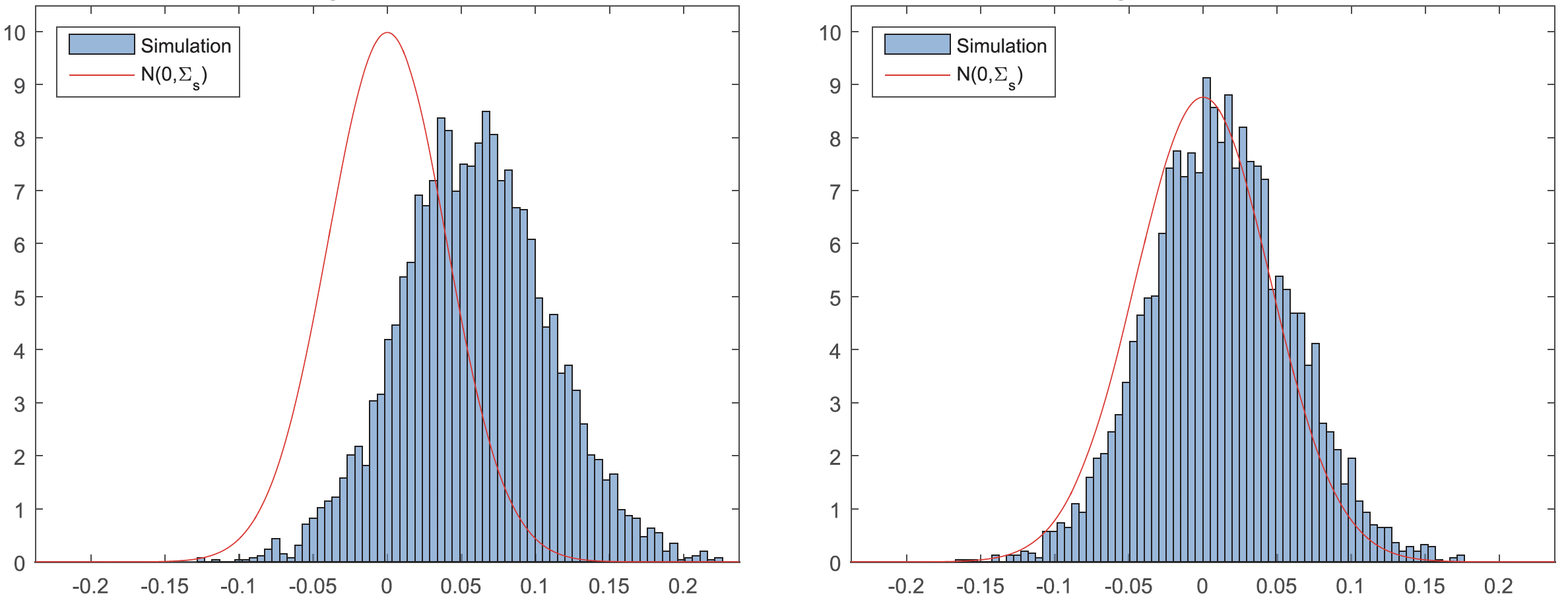
The figure below compares the histograms of the estimation error of $\delta$ for:

• The conventional machine learning estimator (left); and
• The debiased machine learning estimator (right)

in the simulation study in Chernozhukov et al. (2018), where $\mu^{(0)}(x)$ and $p(x)$ are learned by using random forests. The debiased-ML estimator centered better around zero, meaning it has a smaller estimation bias.