Bagging Reduces Estimation Variance #

Bootstrap aggregating (or, in short, bagging) is a computationally intensive method for reducing the variance of unstable estimators. The idea is to aggregate the predictions by a committee of unstable estimators rather than using a single one:

• By bootstrapping we mean drawing $n^*$ data points randomly from the original database $$S=\{Y_i,X_i: i=1,\ldots, n\}.$$ We draw with replacement, allowing the same data points to occur more than once in the resampled dataset.
• Repeat the step above $M$ times to extract the bootstrap samples $$S_m^{*}=\{Y_i^{*},X_i^{*}: i=1,\ldots, n^{*}\},\\~m=1,\ldots,M.$$ Note that we are not generating new data points beyond the original ones, and therefore data sets $S_m^{*}$ are dependent by using the same original database $S$.
• Fit a base estimator $\widehat{f}_m(x)$ to every bootstrap sample $S_m^{*}$ and output the ensemble estimator $$\widehat{f}(x)=\frac{1}{M}\sum_{m=1}^{M}\widehat{f}_m(x).$$
• Bagging uses $n^*=n$ unless specified otherwise.

Bagging Is Not Boosting #

Bagging and boosting are both ensemble learning methods that aggregate many base learners. However, there are at least five crucial differences:

1. Bagging involves randomization, while the (modern) boosting methods are usually deterministic algorithms.
2. Bagging generates base estimators without ordering, whereas boosting generates base estimators sequentially.
3. Bagging uses strong base learners in contrast to the weak base learners used by boosting. Bagging performs very poorly with stumps.
4. Bagging does not require an additive model.
5. Bagging should run forever with a $M$ as large as possible, but we must stop boosting early to avoid overfitting (although it happens slowly).

Bagging Is Smoothing #

Consider again our toy example of unstable estimator. Let $\bar{X}_m^{*}$ denote the $m$-th bootstrap average with $n^*=n$. The bagging estimator for this example is given by

$$\widehat{f}(x)=\frac{1}{M}\sum_{m=1}^{M}\mathbf{1}[\bar{X}_m^*\leq x].$$

By law of large numbers conditioning on the original data set $S$, for large $M$ $$\widehat{f}(x)\approx \mathbb{P}(\bar{X}^*\leq x\mid S),$$ where the variable $\bar{X}^{*}$ represents a generic bootstrap average that has a conditional mean $\bar{X}$ given $S$.

If the bootstrap principle applies, that is, if our resampling mechanism from a given sample $S$ mimics the sampling mechanism of $S$ from the population, then uniformly for $t\in\mathbb{R}$ $$\begin{align*}&\mathbb{P}(\sqrt{n}(\bar{X}^{*}-\bar{X})\leq t\mid S)\\\approx &~\mathbb{P}(\sqrt{n}(\bar{X}-\mu)\leq t)=\Phi(t),&\end{align*}$$ where $\Phi$ denotes the standard normal distribution function. The last equality holds because $\bar{X}\sim N(\mu,1/n)$.

Substituting $t=\sqrt{n}(x-\bar{X})$, $$\begin{align*}&\mathbb{P}(\bar{X}^{*}\leq x\mid S)\\=&~\mathbb{P}(\sqrt{n}(\bar{X}^{*}-\bar{X})\leq \sqrt{n}(x-\bar{X}))\\\approx&~\Phi(\sqrt{n}(x-\bar{X})).\end{align*}$$ Now define $$c(x)=\sqrt{n}(x-\mu)$$ and $$Z=\sqrt{n}(\bar{X}-\mu)\sim N(0,1).$$ It follows that, for large $M$, $$\widehat{f}(x)\approx\Phi(\sqrt{n}(x-\bar{X}))=\Phi(c(x)-Z)$$

Comparing with the unstable estimator $$\widehat{f}(x)=\mathbf{1}[\bar{X}\leq x]=\mathbf{1}[Z-c(x)\leq 0],$$ we observe that bagging smooths the indicator function $\mathbf{1}[u\leq 0]$ to be $\Phi(-u)$.

The figure below illustrates the smoothing effect:

• The solid line is the indicator function $\mathbf{1}[u\leq 0]$; and
• The dotted line is the smoothed function $\Phi(-u)$.

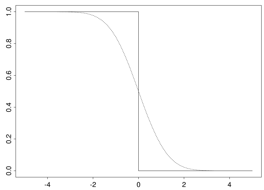
The function $\Phi(-u)$ is continuous in $u$ with a bounded derivative such that $$\begin{align*}\left|\frac{d}{du}\Phi(-u)\right|=&\left|-\phi(-u)\right|\\=&\phi(-u)\leq\phi(0)=\frac{1}{\sqrt{2\pi}},\end{align*}$$ where $\phi$ is the standard normal density function given by $$\phi(x)=\frac{1}{\sqrt{2\pi}}e^{-x^2/2}.$$

A small change, say, $\delta$ in $Z$ can only result in a small change in the estimator in the sense that (using a first-order Taylor expansion) $$\sup_{c\in\mathbb{R}}|\Phi(c-(Z+\delta))-\Phi(c-Z)|\leq \frac{|\delta|}{\sqrt{2\pi}},$$ where the upper bound is nonrandom and tends to 0 as $|\delta|\rightarrow 0$.

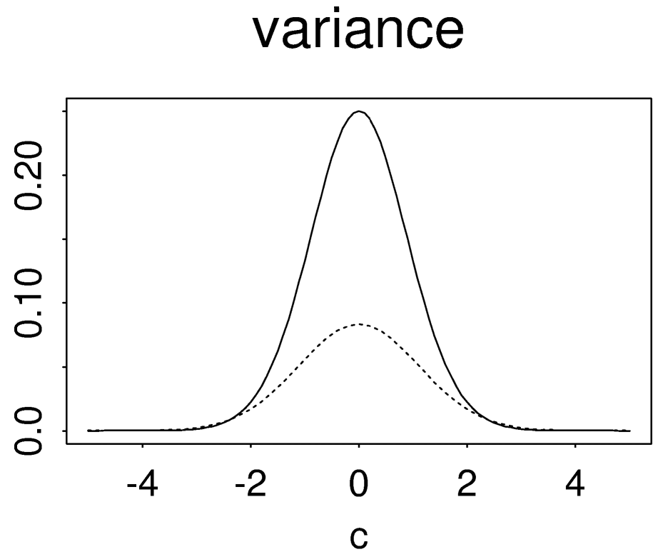
The smoothing effect leads to a significant reduction in the estimation variance. At the most unstable point $x=\bar{X}$ with $c(x)=0$, the unstable estimator has the variance $$\operatorname{var}(\mathbf{1}[Z\leq 0])=\frac{1}{4}$$ whereas the bagging estimator has only a limiting variance (as $M\rightarrow\infty$) of $$\operatorname{var}(\Phi(-Z))=\operatorname{var}(U)=\frac{1}{12},\\U\sim\operatorname{Unif}(0,1).$$ Below is a plot of their variances as a function of $c$. The solid line is for the unstable estimator $\mathbf{1}[Z-c\leq 0]$ and the dashed line is for the limit of the bagging estimator $\Phi(c-Z)$.