Subagging with Trees #

Like for our toy example of the unstable estimator, instability also arises in decision trees grown by CART because of the ‘hard’ decisions with indicators made by the splits. To improve stability, one can smooth the prediction by aggregating unstable CART trees predictions using bagging.

Regarding computational costs (and sometimes technical reasons), one might want to draw data points without replacement from the original data. This means we must draw fewer data points with $n^{*}<n$; otherwise, we duplicate the sets in the resampling procedure, and no smoothing effect can emerge. This approach is usually called subsample aggregating or subagging in short.

The fraction subagging uses $n^*=[na]$ with some fraction $a\in (0,1)$; A particular case is the half subagging with $a=1/2$.

The small-order subagging uses much less data points such that, in theory, the ratio between $n^*$ and $n$ vanishes to zero, that is, $n^{*}/n\rightarrow 0$ as $n\rightarrow\infty$. In this case, we can still draw data points with replacement if we wish as there is only a small chance to draw the same observation twice or more. There is little difference between whether we draw with or without replacement. For example, the causal forest algorithm often uses small-order subagging with replacement.

Decorrelating the Trees #

The bagging and subagging estimators we discussed are consistent with the original definition of random forest in Breiman (2001) although we focus on regression rather than classification tasks:

A random forest is a classifier consisting of a collection of tree-structured classifiers $h(x,\Theta_m|S)$ where $\Theta_m$ are independent identically distributed random vectors and each tree is fully grown.

The parameters $\Theta_m$ include, for example, the random draws of observations in resampling.

Nowadays, random forest usually means a regularized version of the (su)bagging estimator: when generating the pool of candidate splits, only a random sample of $\widetilde{d}<d$ features is allowed for each split. For example, one might use $\widetilde{d}=\sqrt{d}$.

We emphasize that the decision trees are correlated even if the bootstrap data sets are drawn independently from a common training data set. The (positive) correlations may significantly increase the estimation variance and undermine the smoothing effect of bagging. The additional randomness in random forest decorrelates the trees by enforcing the trees to consider different pools of candidate splits and leads to better variance reduction.

Honest Trees #

Below is a heatmap of the random forest predictions from Wager (2016) with two uniformly distributed features $X=(X_1,X_2)\in [0,1]^2$ but the target $Y$ is independent of $X$. The prediction are consistently darker near the edges, meaning the random foreast systematically makes larger predictions around the boundaries.

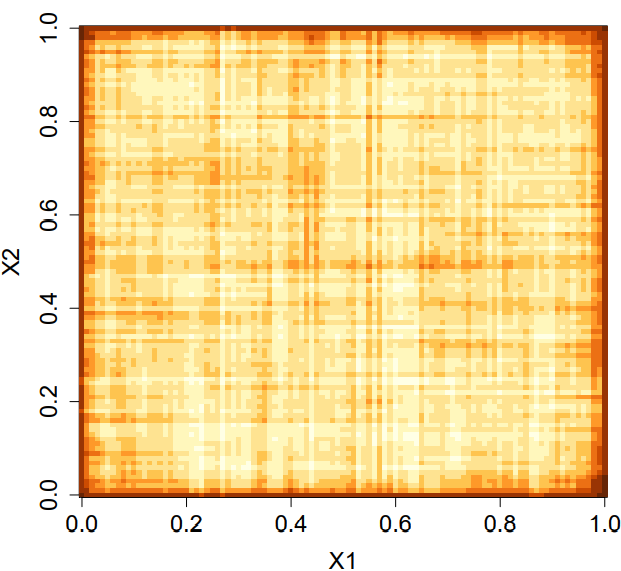
This boundary issue is not desirable as the optimal prediction rule should be constant because of the independence between the target and features. It turns out the problem is because CART trees are not ‘honest’ in the sense that it determines splits and prediction simultaneously using the same data set.

To attack the boundary issues for independent data, one may split the data into halves: use one half to find splits, and the other half to make predictions. Using honest trees can avoid the dependence between splits and predictions and remove bias in estimation. A more general version, called cluster-robust random forests, is available in Athey and Wager (2019).