Structral Equations #

Suppose that the invididual treatment effect is a fixed constant given by $$\delta_i=Y_i^{(1)}-Y_i^{(0)}\equiv\delta.$$ Note that this is also the ATE $\tau=\delta$ and the CATE $\tau(x)\equiv\delta$. Moreover, assume that the potential outcome in the control group $Y_i^{(0)}$ obeys a linear regression model on confounders $X_i=(X_{i1},\ldots, X_{id})$ given by $$Y_i^{(0)}=\sum_{j=1}^{d}X_{ij}\beta_j+\varepsilon_i,$$ where we omit the intercept for simplicity and $\varepsilon_i$ are zero-mean errors independent of the confounders $X_i$ and treatment dummy $D_i$.

Combining the last two equations yields the linear regression model for the outcome $$Y_i=\delta D_i+\sum_{j=1}^{d}X_{ij}\beta_j+\varepsilon_i.$$ On the other hand, without loss of generality, we can always decompose $$D_i=p(X_i)+v_i,\quad \mathbb{E}[v_i|X_i]=0,$$ where $p(x)=\mathbb{E}[D_i|X=x]$ denotes the conditional propensity score.

Collecting both information on the outcome $Y$ and the treatment $D$ yields the structural equations $$\begin{cases}Y_i=\delta D_i+\sum_{j=1}^{d}X_{ij}\beta_j+\varepsilon_i&\\D_i=p(X_i)+v_i\end{cases}$$ where $$\mathbb{E}[\varepsilon_i|X_i,D_i]=0,~\mathbb{E}[v_i|X_i]=0.$$ Note that $\varepsilon_i$ and $v_i$ are uncorrelated.

Double Selection #

First, let us consider only the regression model for the outcome (i.e., the first equation in the structural model). When the dimension $d$ is large (relative to the sample size $n$), the least-squares estimator of the treatment effect $\delta$, controlling $X_i$, may suffer from large estimation variance or even inconsistency.

Let us define the support of the outcome regression coefficients as the index set of the relevant features with $\beta_j$ given by $$T_1=\{1\leq j\leq d: \beta_j\neq 0\}.$$ This set is sparse if it only contains a few elements or at least much less than the sample size $n$. If $T_1$ were known with size $|T_1|/n\approx 0$, one can overcome the dimensionality issue for least-squares estimation by omitting irrelevant features. This approach is called post-selection least-squares estimation.

In practice, one may estimate $T_1$ by the set of active variables, say, $$\widehat{T}_1=\{1\leq j\leq d: \widehat{\beta}_j\neq 0\}$$ selected by the LASSO regression with an appropriate penalty coefficient such that, with high probability $$T_1\subset\widehat{T}_1$$ and for some constant $C\geq 1$ $$|\widehat{T}_1|\leq C |T_1|\ll n.$$ Note that the set estimator $\widehat{T}_1$ needs not be consistent towards $T_1$. The first property only requires that it does not miss relevant features. The second property allows it to include irrelevant features by mistakes as long as the impact is not overwhelming.

Bias and non-normality issues can still arise as there is a small chance that the estimated set $\widehat{T}_1$ misses some important confounders. One may want to extend $\widehat{T}_1$ in some sense to reduce such mistakes, but we must be cautious not to overextrapolate the support set. One obvious way is to include the confounders that the researchers believe are necessary, say, $\widehat{T}_0$ if available. Another way is to incorporate the information from treatment, the second equation in the structural models.

For all practical purposes, suppose we can approximate the conditional propensity score by a linear probability model $$p(X_i)=\sum_{j=1}^{d}X_{ij}\gamma_j+r_i$$ where the approximation errors $r_i$ are sufficiently small in probability. Then we can also apply LASSO regression to the treatment dummy on the confounders to get another set $$\widehat{T}_2=\{1\leq j\leq d:\widehat{\gamma}_j\neq 0\}.$$

Finally, we choose the features in the set union $\widehat{T}=\widehat{T}_0\cup \widehat{T}_1\cup\widehat{T}_2$. The extended set $\widehat{T}$ may still satisfy the two desirable properties above as for $\widehat{T}_1$, but with a smaller probability to miss important confounders. This selection appraoch is called double LASSO method or double selection method, as we need to select variables in both structral equations.

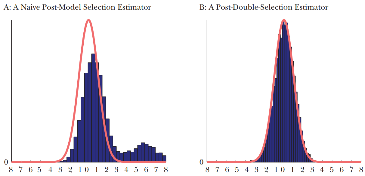
The following figure from Belloni et al. (2013) demonstrates at least two potential benefits of the double selection for the studentized estimators:

• the bias of the post-selection estimator is small(er);
• the distribution of the post-selection estimator is closer to normal.