Architecture of a Traditional CNN #

A convolutional neural network is composed of at least 3 layers:

• A convolution layer to perform convolution operations and to generate many feature maps from one image;
• A pooling layer to denoise the feature maps by shrinking non-overlapping submatrices into summary statistics (such as maximums);
• A dense layer which is a usual (shallow/deep) neural network that takes flattened inputs.

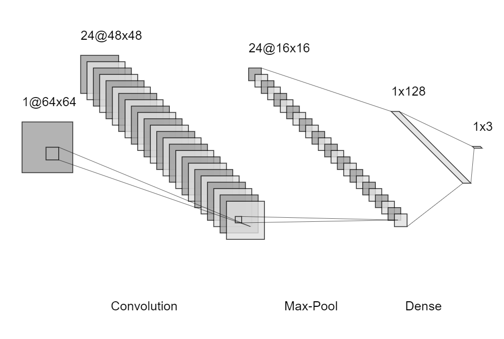
In general, one may create different combinations of the convolution and pooling layers. For example, one may multiple convolution layers before a pooling layer. One may also apply several successive pairs of such layers.

Convolution Layer #

Here is an example to illustrate how to apply convolution operation.

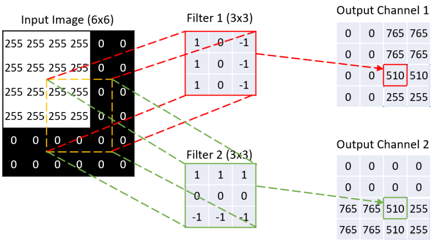
• On the left is an input image represented as a matrix (255=white, 0=black) given by $$\boldsymbol{V}=\{V_{\mathrm{i},\mathrm{j}}:\mathrm{i}=1,\ldots,\mathrm{I}, ~\mathrm{j}=1,\ldots,\mathrm{J}\}.$$In our example, $\mathrm{I}=\mathrm{J}=6$.

• In the middle there are two kernel matrices (or just kernels), each corresponding to a filter. Denote the kernel matrices by $$\boldsymbol{W}_{\mathrm{k}}=\{W_{\mathrm{k},\mathrm{s},\mathrm{t}}:1\leq\mathrm{s}\leq \mathrm{S},~1\leq \mathrm{t}\leq \mathrm{T}\}$$ for $1\leq k\leq K$, where $K$ denotes the number of filters. In our example, $\mathrm{S}=\mathrm{T}=3$.

• For each filter, we cycle through the subregions of $\boldsymbol{V}$ of the same size $$\begin{align*}\boldsymbol{V}^{(\mathrm{i},\mathrm{j})}=\{V_{{\mathrm{i}+\mathrm{s}-1,\mathrm{j}+\mathrm{t}-1}}:&1\leq \mathrm{s}\leq \mathrm{S},\\&1\leq \mathrm{t}\leq \mathrm{T}\}\end{align*}$$ and output a set of matrices $$\begin{align*}\boldsymbol{A}_{\mathrm{k}}=\{A_{\mathrm{k},\mathrm{i},\mathrm{j}}: &1\leq \mathrm{i}\leq \mathrm{I}-\mathrm{S}+1,\\&1\leq \mathrm{j}\leq \mathrm{J}-\mathrm{T}+1\}\end{align*}$$ where $$\begin{align*}A_{\mathrm{k},\mathrm{i},\mathrm{j}}=&\left( \text{vec}(\boldsymbol{W}_{\mathrm{k}})\right)^T \text{vec}(\boldsymbol{V}^{(\mathrm{i},\mathrm{j})})\\ =&\sum_{\mathrm{s},\mathrm{t}}W_{\mathrm{k},\mathrm{s},\mathrm{t}}V_{\mathrm{i}+\mathrm{s}-1,\mathrm{j}+\mathrm{t}-1}.\end{align*}$$ We drop the convolutions near the edges if dimensions do not match. For other padding options, we refer to here.

• Next, we add bias terms $w_{\mathrm{k},0}$ to filtered features $\boldsymbol{A}_1,\ldots,\boldsymbol{A}_K$ and apply activation $\sigma$ to get the feature maps $$\boldsymbol{Z}_{\mathrm{k}}=\sigma(\boldsymbol{A}_{\mathrm{k}}+w_{\mathrm{k},0})$$ where $\sigma$ should be applied entry-wisely. On the right of the example figure above shows the feature maps with no bias terms and $\sigma$ as the ReLU function.

In our example, we specify the kernal matrices and bias terms already. In practice, they are the parameters we need to fit.

Pooling Layer #

The collection of feature maps $\{\boldsymbol{Z}_{\mathrm{k}}: k=1,\ldots, K\}$ has a much larger dimension than the original input image. Flattening them directly without extra treatments is not intelligent, as the dimensionality issue may degrade the statistical performance. Furthermore, if the signals are relatively sparse, the convolution operation may reduce the signal strength by mixing signals and noises. We usually add an additional pooling layer after convolution to reduce the data dimension and denoise the feature maps.

The idea is to split the feature maps into non-overlapping divisions and replace each division with a summary statistic. A popular approach is the max-pooling, which replaces each squared block with the maximum of its entries. The length of the sides $S$ is usually called the stride. An underlying assumption is that a more significant value (a lighter pixel) means a stronger signal. The following figure illustrates the max-pool operation for our example above:

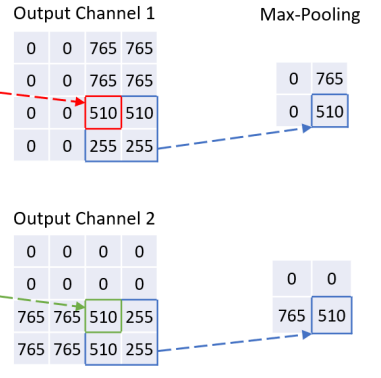
Note that there is no parameter needed once we have chosen the stride $S$.

Dense Layer #

Finally, we flatten the feature maps after pooling and input them into an ordinary neural network (being it shallow or deep). As the signal should be relatively dense after pooling, we use a fully connected network.