Deep Neural Networks #
We can construct feedforward neural networks $f(x):\mathbb{R}^d\rightarrow\mathbb{R}^K$ with more hidden layers as follows.
Denote the input of size $M_0=d$ to the neural net by $$z^{(0)}=\begin{pmatrix}x_1\\\vdots\\x_d\end{pmatrix}\in\mathbb{R}^{d}.$$ We compute $M_1$ activations making up the first hidden layer by $$z^{(1)}=\sigma(a^{(1)}),\quad a^{(1)}=W^{(1)}z^{(0)}+b^{(1)}$$ where $W^{(1)}\in\mathbb{R}^{M_1\times M_0}$ is a matrix of weights and $b^{(1)}\in\mathbb{R}^{M_1}$ is a vector of biases. We apply the activation function $\sigma$ element-wisely to the vector $a^{(1)}$.
Treating $z^{(1)}$ as the input for next hidden layer, we can construct $M_2$ new activations $$z^{(2)}=\sigma(a^{(2)}),\\ a^{(2)}=W^{(2)}z^{(1)}+b^{(2)},$$ where $W^{(2)}\in\mathbb{R}^{M_2\times M_1}$ is the matrix of weights, $b^{(2)}\in\mathbb{R}^{M_2}$ is the vector of biases, and $\sigma$ is usually the same activation function as above.
Repeating the procedure above for $l=3,\ldots, D-1$ (if $D\geq 4$) to construct as many hidden layers as wish: $$z^{(l)}=\sigma(a^{(l)}),\\ a^{(l)}=W^{(l)}z^{(l-1)}+b^{(l)},\\ $$ where $l$ is the index of the layer and $D$ is the depth of the neural net. Let $M_l$ denote the number of hidden units in the $l$-th hidden layer, and then $W^{(l)}\in\mathbb{R}^{M_l\times M_{l-1}}$ are matrices of weights and $b^{(l)}\in\mathbb{R}^{M_l}$ are vectors of biases.
The $K$-dimensional output is given by $$f(x)=\boldsymbol{\sigma}(a^{(D)}),\\ a^{(D)}=W^{(D)}z+b^{(D)}$$ where $W^{(D)}\in\mathbb{R}^{M_D\times M_{D-1}}$ is the matrix of weights with $M_D=K$ and $b^{(D)}\in\mathbb{R}^{M_D}$ is the vector of biases. The function $\boldsymbol{\sigma}(x)=x$ can be identity for regression problems, the softmax $\boldsymbol{\sigma}(x)=\operatorname{SoftMax}(x)$ for classification problems, or just an(other) activation function.
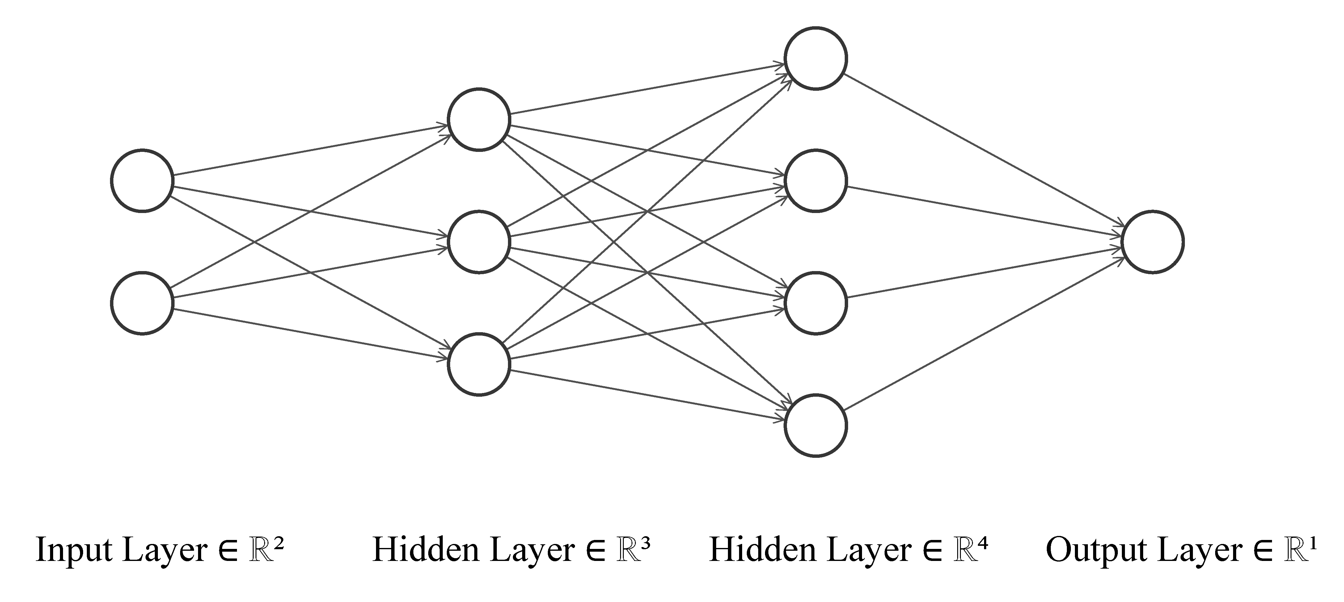
When $D=1$, there is no hidden layer and we have the linear models. When $D=2$, we obtain the shallow neural network in the last chapter. We refer deep neural networks for those with depth $D\geq 3$. The following illustrates a single-output neural networks with depth $D=3$.

How Deep Should It Be? #
In finance applications, however, the depth is usually no more than 6. For monthly equity returns, $D=3$ is a good choice; see, e.g., Gu et al. (2019). In theory, the depth $D$ should grow slowly to infinity with the sample size at the order of $\log(n)$, for instance. Even with 1.2 million training images in AlexNet, for example, the depth $D$ should be only a multiple (or a fraction) of $\log (1.2\times 10^6)\approx 14$.
The deep neural networks share a similar universal approximation property as the shallow neural networks: for a sufficiently large number of hidden units and depth, there exists a deep neural network approximating a smooth regression function arbitrarily well. We do not pursue the technical details here.
Benefits of Deep Neural Networks #
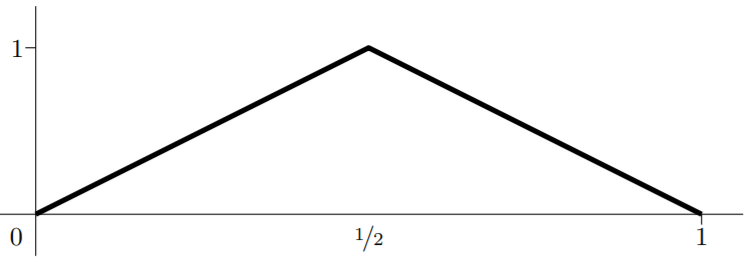
Consider the following so-called mirror-map function from Telgarsky (2015):
$$m(x):=\begin{cases}2 x & 0 \leq x \leq 1 / 2 \\2(1-x) & 1 / 2<x \leq 1 \\0 & \text { otherwise }.\end{cases}$$
Below is the plot of $m(x)$ for $x\in[0,1]$.
 We can express the mirror map as a shallow neural network in form of
$$m(x)=\sigma(W_2\sigma (W_1x+b_1)),$$
where $\sigma(x)=\operatorname{ReLU}(x)$ is the ReLU activation function, $W_1$ and $W_2$ are some known weight matrices, and $b_1$ is some known bias vector.
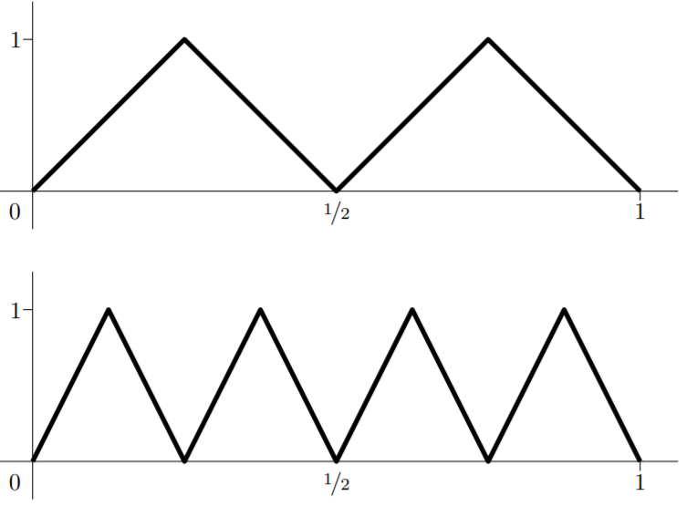
Now consider the regression function $$\mu(x):=\underbrace{m(m(\cdots (m}_{k~\text{times}}(x))\cdots)),$$ which is a deep neural network with depth $L=2k$ and a total number of parameters growing only linearly in $k$ as $k\rightarrow\infty$. Below is the plot of $\mu(x)$ for $k=2$ and $k=3$ on $[0,1]$.

On the other hand, expressing the same function $\mu(x)$ using shallow neural networks requires at least $2^k-1$ hidden units, meaning that the total number of parameters must grow exponentially in $k$. Hence, for large $k$, the deep neural network requires much less parameters.
In general, deep neural networks provide the opportunities to tradeoff width and depth to reduce the number of units required for the same approximation error. This will reduce the total number of parameters to be estimated and improve the statistical performance of our fitted network.