Decision Tree #
A decision tree grows from a root representing a YES/NO condition. The root branches into two child nodes for two different states. We travel from the root to its left child node when the condition is true or otherwise to its right child. Each child node could be a leaf (also called terminal node) or the root of a subtree. For the latter case, we continue growing and traveling until we reach a terminal.
All the nodes except the terminal ones represent conditions; it has become a common practice that each of them should be on only one of the features. We output a decision or a prediction at each leaf. The following figure illustrates a decision tree with 5 leaves.
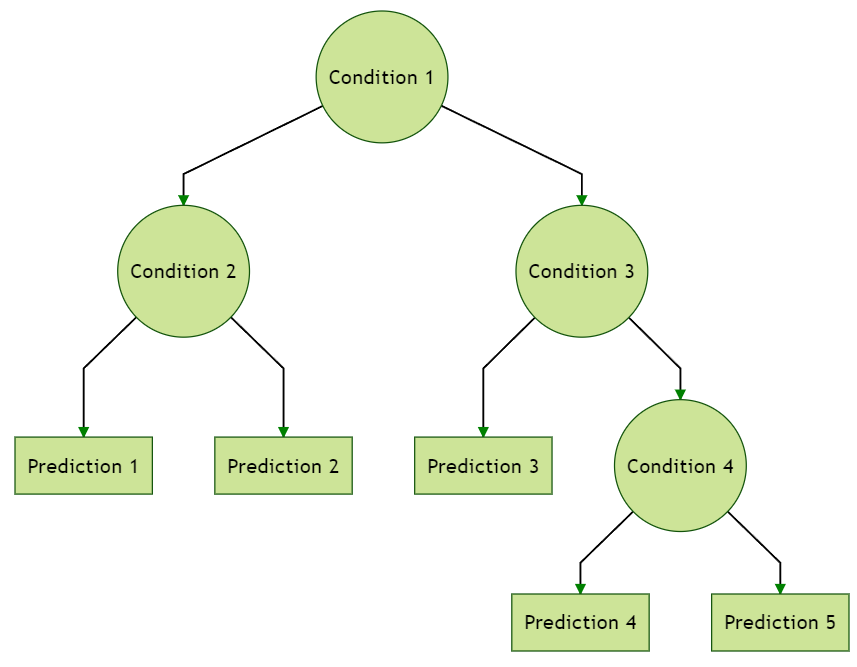
The depth of a tree is the maximum number of steps to travel from its root to the leaves. The example tree above has a depth of 3.
Classification And Regression Tree (CART) Algorithm #
We shall only explain how the CART algorithm finds the first split for the root node. Then we repeat splitting sequentially for every internal node as a subtree’s root until a stopping criterion is reached. This approach is called recursive binary splitting.
First, generate a large pool of candidate splits represented by $$\{(j^{(b)},\alpha^{(b)}):b=1,\ldots,B\}$$ where $j^{(b)}\in\{1,\ldots,d\}$ is a feature index, $\alpha^{(b)}\in (0,1)$ is a probability threshold level, and $b$ is the index for a candidate split.
For every split with index $b$, partition the input feature space $\mathcal{X}\subset\mathbb{R}^d$ into two sub-regions: $$\mathcal{X}_L^{(b)}=\{x\in\mathcal{X}: x_{j^{(b)}}<\theta^{(b)}\}\\\mathcal{X}_R^{(b)}=\{x\in\mathcal{X}: x_{j^{(b)}}\geq\theta^{(b)}\}$$ The quantile threshold level $\theta^{(b)}$ equals to the sample quantile of the $j^{(b)}$-th feature at level $\alpha^{(b)}$.
Denote the subset of target points belonging to the left child $\mathcal{X}_L^{(b)}$ by $$\mathcal{Y}_L^{(b)}=\{Y_i\in\mathcal{Y}: X_i\in\mathcal{X}_L^{(b)}, 1\leq i\leq n\}$$ and, similarly, define that for the right child $\mathcal{X}_R^{(b)}$ by $$\mathcal{Y}_R^{(b)}=\{Y_i\in\mathcal{Y}: X_i\in\mathcal{X}_R^{(b)},1\leq i\leq n\}.$$ We compute the impurity of each subset $\mathcal{Y}_{\tau}$, $\tau\in\{L,R\}$, using some impurity function $\psi$ to be specified later on. Heuristically, if the data points in the sub-region $\mathcal{Y}_{\tau}$ spread out more, then we have a larger impurity value $\psi(\mathcal{Y}_{\tau}).$ We assess the weighted sum of impurity over both children given by $$p_L^{(b)}\psi(\mathcal{Y}_L^{(b)})+p_R^{(b)}\psi(\mathcal{Y}_R^{(b)})$$ with the (sample) probabilities $$p_L^{(b)}=\frac{|\mathcal{X}_L^{(b)}|}{|\mathcal{X}|},\quad p_R^{(b)}=\frac{|\mathcal{X}_R^{(b)}|}{|\mathcal{X}|}$$ where $|A|$ denotes the number of elements in a set $A$.
We choose the split $b^*$ with the smallest weighted total impurity given by
$$b^*=\underset{b\in\{1,\ldots,B\}}{\operatorname{argmin}}~ \left( p_L^{(b)}\psi(\mathcal{Y}_L^{(b)})+p_R^{(b)}\psi(\mathcal{Y}_R^{(b)})\right).$$
Choosing the Impurity Function #
The difference between regression trees and classification trees is their choice of impurity functions. The regression tree uses an impurity function that is more suitable for a target variable with ordered values (think of a continuous target variable, for example). In particular, for regression trees we often use the variance statistic, namely,
$$\psi(\mathcal{Y}_{\tau})=\operatorname{var}(\mathcal{Y}_{\tau})=\frac{1}{|\mathcal{Y}_{\tau}|}\sum_{Y_i\in \mathcal{Y}_{\tau}}(Y_i-\bar{Y}_{\tau})^2\\\bar{Y}_{\tau}=\frac{1}{|\mathcal{Y}_{\tau}|}\sum_{Y_i\in \mathcal{Y}_{\tau}}Y_i.$$
Here we remove the superscript $b$ for convenience of presentation.
For a classification tree with a $K$-class target variable, we may rather use the cross-entropy
$$\psi(\mathcal{Y}_{\tau})=\sum_{k=1}^{K}-\log p_{\tau k}\cdot p_{\tau k}$$
where $(p_{\tau 1},\ldots,p_{\tau K})$ denotes the sample distribution of the labels in the set $\mathcal{Y}_{\tau}$ given by
$$p_{\tau k}=\frac{|\mathcal{Y}_{\tau}\cap \{\mathcal{C}_k\}|}{|\mathcal{Y}_{\tau}|}$$ where $\mathcal{C}_k$ denotes the $k$-th label. Note that here we allow the same target value occurs more than once in the data set.
From the unified view of regression and classification, we could also treat the classification problem as a regression problem for the one-hot encoded target varibles $$(Y^{(1)},\ldots,Y^{(K)}),\quad Y^{(k)}=\mathbf{1}[Y= \mathcal{C}_k].$$ What happens if we now use the variance statistic as for the regression tree? Let us sum up the variance statistics over the binary entries of the one-hot encoded target vectors, then we obtain the Gini index given by $$\begin{align*}\psi(\mathcal{Y}_{\tau})=& \sum_{k=1}^{K}p_{\tau k}(1-p_{\tau k})\\=&1-\sum_{k=1}^{K}p_{\tau k}^2.\end{align*}$$
Forecasting With Decision Trees #
The leaves (or, terminal nodes) partition the entire feature space into $\Tau$ disjoint subregions $\mathcal{R}_{\tau}$, $\tau=1,\ldots,\Tau$, such that $$\mathcal{X}=\cup_{\tau=1}^{\Tau}~ \mathcal{R}_{\tau}$$ and $$\mathcal{R}_{\tau}\cap \mathcal{R}_{\tau'}=\emptyset,~\tau\neq \tau'.$$ Our prediction rule is then a $\Tau$-terminal node tree (if $x\in\mathcal{R}_{\tau}$, then predict $c_{\tau}$), however, usually with a large $\Tau$ such that $$f(x)=\sum_{\tau=1}^{\Tau}c_{\tau}\mathbf{1}(x\in \mathcal{R}_{\tau})$$ and our node-wise predictions are simply the sample average of the target values given by $$c_{\tau}=\frac{\sum_{i=1}^{n} Y_i\mathbf{1}[X_i\in\mathcal{R}_{\tau}]}{\sum_{i=1}^{n} \mathbf{1}[X_i\in\mathcal{R}_{\tau}]}.$$ For a classification problem, one should replace the target variable in the last line with its one-hot encoded vectors such that $$c_{\tau}=(c_{\tau 1},\ldots,c_{\tau K})$$ with $$\begin{align*}c_{\tau k}=&\frac{\sum_{i=1}^{n} Y_i^{(k)}\mathbf{1}[X_i\in\mathcal{R}_{\tau}]}{\sum_{i=1}^{n} \mathbf{1}[X_i\in\mathcal{R}_{\tau}]}\\=&\frac{\sum_{i=1}^{n} \mathbf{1}[Y_i=\mathcal{C}_k,~X_i\in\mathcal{R}_{\tau}]}{\sum_{i=1}^{n} \mathbf{1}[X_i\in\mathcal{R}_{\tau}]}.\end{align*}$$ In this case, $c_{\tau}=(c_{\tau 1},\ldots,c_{\tau K})$ represents a prediction of the (conditional) label distribution.
For a single classification tree, one may consider a majority vote within each terminal node and output the Bayes classifier immediately rather than a distribution. However, we will not focus on a single tree but aggregate many trees. We should aggregate the distribution prediction rather than the majority votes for stability concerns. Hence, most computer packages for the random forest have abolished the majority voting approach. In other words, the modern practice is to treat classification tasks as regression tasks with one-hot encoded targets.