Why Nonlinear Models #

Consider a scalar target variable $Y\in\mathbb{R}$ and two independent dummy features $$X=(X_1,X_2)\in\{0,1\}^2.$$Suppose that $$\mathbb{P}(X_j=1)=\mathbb{P}(X_j=0)=0.5,~j\in\{1,2\},$$ and the true regression function equals to the Exclusive Or (XOR) function given by $$\mu(x)=\mathbf{1}[x_1\neq x_2].$$

However, we do not know this population regression function but restrict ourselves to the linear models for convenience. In other words, we only consider the predition rule $f$ from the space $$\begin{align*}\mathcal{H}=\{ &f(x;\theta)=\beta_1x_1+\beta_2x_2+\beta_0:\\& \theta=(\beta_0,\beta_1,\beta_2)\in\mathbb{R}^{3}\}\end{align*}$$ which excludes the XOR function unfortunately.

For each candidate function $f=f(\cdot;\theta)\in\mathcal{H}$, we can decompose the expected squared loss by

$$\begin{align*}&\mathbb{E}[(f(X;\theta)-Y)^2]\\=&\mathbb{E}[(f(X;\theta)-\mu(X))^2]\\&+\underbrace{\mathbb{E}[(\mu(X)-Y)^2]}_{\text{not depending on}~ \theta}\end{align*}$$

Minimizing the first term $$ \begin{align*} &\mathbb{E}[(f(X;\theta)-\mu(X))^2]\\=&\frac{1}{4}\Bigg\lbrace(\beta_0-0)^2+(\beta_0+\beta_1-1)^2\\&+(\beta_0+\beta_2-1)^2+(\beta_0+\beta_1+\beta_2-0)^2 \Bigg\rbrace\end{align*}$$ yields the solution $(\beta_0,\beta_1,\beta_2)=(1/2,0,0)$, corresponding to the ideal linear prediction rule $f^{*}(x)=1/2\neq \mu(x)$.

Feedforward Networks #

We need a nonlinear model to express the XOR function. In particular, consider any function $f:\mathbb{R}^{d}\rightarrow\mathbb{R}$ of the following form:

$$f(x)=\sum_{m=1}^{M}w_{1,m}^{(2)}z_m+b^{(2)},~ z_m=\sigma\left( a_m^{(1)}\right),\\ a_m^{(1)}=\sum_{j=1}^{d}w_{m,j}^{(1)}x_j+b_m^{(1)},~x= (x_1,\ldots,x_d)\in\mathbb{R}^{d}.$$

This class of functions is called feedforward neural networks:

• Extending the notation of sigmoid function $\sigma$, the function $\sigma$ here refers to any activation function chosen by the user.
• The parameters $w_{m,j}^{(1)}$ and $w_{1,m}^{(2)}$ are called weights.
• The parameters $b_m^{(1)}$ and $b^{(2)}$ are called biases, not to be confused with the bias of an estimator in statistics.

The set of input units $x_j$ forms the input layer, and the set of hidden units $z_m$ forms a hidden layer.

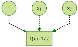
When $\sigma(x)=x$, or any linear function with a nonzero slope, the hidden layer is superfluous and the feedforward network reduces to a linear model. The following figure illustrates the optimal linear prediction rule $f(x)=1/2$ for the XOR function (the dotted links means zero weights):

In contrast, the following figure shows the representation of the XOR function as a feedforward network using the Rectified Linear Unit (ReLU) activation function $\operatorname{ReLU}(x)=\max\{0,x\}$.

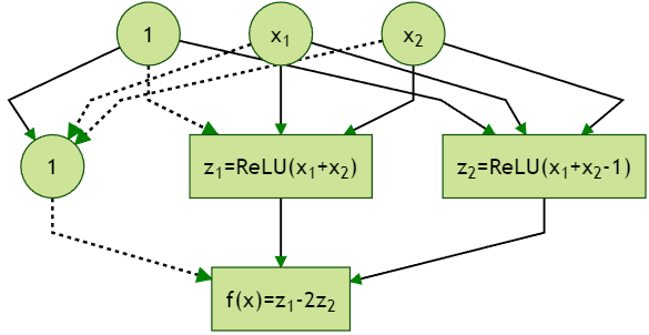
There are three layers in the model: on top is the input layer consisting of input units, in the middle is the hidden layer consisting of hidden units, and at the bottom is the output layer showing the function’s output. We call this type of neural network shallow because there is only one hidden layer.

One can verify the final ouput as follows:

$$ \begin{align*}\begin{cases}x_1=0\\x_2=0\end{cases}\end{align*}\Rightarrow \begin{cases}z_1=0\\z_2=0\end{cases} \Rightarrow f(x)=0$$

$$ \begin{align*}\begin{cases}x_1=1\\x_2=0\end{cases}\end{align*}\Rightarrow \begin{cases}z_1=1\\z_2=0\end{cases} \Rightarrow f(x)=1$$

$$ \begin{align*}\begin{cases}x_1=0\\x_2=1\end{cases}\end{align*}\Rightarrow \begin{cases}z_1=1\\z_2=0\end{cases} \Rightarrow f(x)=1$$

$$ \begin{align*}\begin{cases}x_1=1\\x_2=1\end{cases}\end{align*}\Rightarrow \begin{cases}z_1=2\\z_2=1\end{cases} \Rightarrow f(x)=0$$