The weight decay method is an example of the so-called explicit regularization methods. For neural networks, implicit regularization is also popular in applications for their effectiveness and simplicity despite their less developed theoretical properties. In this section, we discuss three implicit regularization methods.

Stochastic Gradient Descent #

One first example is the stochastic gradient descent (SGD) method. The SGD method uses a minibatch $B_t\subset \{1,\ldots,n\}$ each time to replace the batch gradient $g(w(t),b(t))$ with a minibatch gradient given by

$$g_t(w,b)=\frac{1}{|B_t|}\sum_{i\in B_t} \begin{bmatrix}\nabla_{w}\ell(f(X_i;w,b),Y_i)\\\nabla_{b}\ell(f(X_i;w,b),Y_i)\end{bmatrix}.$$

where $|B_t|$ denotes the number of instances in $B_t$. The best practice is randomly partitioning the whole index set into non-overlapping minibatches of (almost) equal size and cycle through these minibatches per epoch. In this way, we use each training example only once per epoch. One may randomly shuffle the dataset and create new non-overlapping minibatches for each epoch. The SGD is noisier and therefore is better at escaping from the local minimum. It may deliver better statistical performance by regularizing the gradient flow over the path.

Early Stopping #

Another example of implicit regularization is the early stopping method. The idea is not to wait until the convergence of the iterative process but use intermediate parameters $w(\tau)$ and $b(\tau)$ even if it is possible to reduce the errors significantly in the next iteration(s). Choosing the stopping time $\tau$ often requires splitting the data into training and validation sets. The following figure from Goodfellow et al. (2016), Chapter 7, illustrates the different behaviors of training and validation losses over epochs.

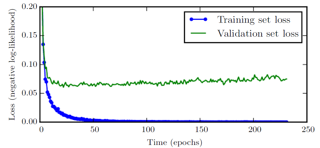
We use the training set to compute gradients and update parameters but evaluate average loss over the validation set. We stop early when the validation set loss is nearly minimal.

Dropout #

Our last example is the dropout method, which sets activations randomly to 0 with a given probability in every step (or epoch). As different sets are used over epochs, all neurons are used in the long run. To aggregate the estimates over different dropout sets, one needs to re-weight the activation accordingly. We omit these technical details but refer to Section 7.12 of Goodfellow et al. (2016).