Shallow Feedforward Networks #

We can stack scalar feedforward networks to allow for multiple outputs. This extension is essential when dealing with multivariate regression functions for one-hot encoded targets. From now on, we call this general form shallow feedforward networks.

A shallow feedforward network is a function $f:\mathbb{R}^{d}\rightarrow \mathbb{R}^K$ of the form:

$$f(x)=\begin{pmatrix}f_{1}(x)\\\vdots\\f_{K}(x)\end{pmatrix} =\boldsymbol{\sigma} \begin{pmatrix}a_{1}^{(2)}(x)\\\vdots\\ a_{K}^{(2)}(x)\end{pmatrix},$$

where we extend the notation of $\boldsymbol{\sigma}:\mathbb{R}^K\rightarrow\mathbb{R}^{K}$ to allow it to be:

• The softmax function $\boldsymbol{\sigma}(a)=\operatorname{SoftMax}(a)$ for classification problems; or
• The identity function $\boldsymbol{\sigma}(a)=a$ for regression problems; or
• $\boldsymbol{\sigma}(a)=(\sigma(a_1),\ldots,\sigma(a_K))^T$ for some element-wise activation $\sigma$.

Without loss of generality, the units ${a_{k}^{(2)}}$ share the same hidden units ${z_m}$ such that

$$a_k^{(2)}(x)=\sum_{m=1}^{M}w_{k,m}^{(2)}z_m(x) +b_k^{(2)}\\z_m(x)=\sigma\left( a_m^{(1)}(x)\right)\\ a_m^{(1)}(x)=\sum_{j=1}^{d}w_{m,j}^{(1)}x_j+b_m^{(1)}$$ where $\sigma$ denotes any activation function (may or may not be the sigmoid). When no confusion arises, we often abbreviate $a_{k}^{(2)}(x)$ and $z_m(x)$ as $a_{k}^{(2)}$ and $z_m$ but bear in mind that they are all functions of the input $x$.

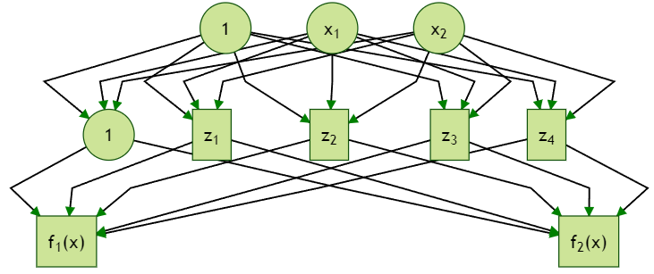
The following figure illustrates an example of two-output shallow feedforward network models with four hidden units (not counting the bias unit). The universal approximation property generalizes for any finite $K$: if one can approximate each coordinate of the $K$-dimensional regression functions arbitrarily well, then it is possible to approximate the multivariate function arbitrarily well.

Choosing the Activation Function #

How do we choose the activation function? A popular choice in modern practice is the ReLU function used before for representing the XOR function given by $$\operatorname{ReLU}(a)=\max\{0,a\}.$$ A more traditional choice is the sigmoid function $$\operatorname{Sigmoid}(a)=\frac{1}{1+\exp(-a)}$$ or the hyperbolic tangent function given by $$ \tanh(a)=\frac{\exp(a)-\exp(-a)}{\exp(a)+\exp(-a)}.$$

Below are the plots of the ReLU, sigmoid and hyperbolic tangent functions. All functions are increasing: ReLU is piecewise linear while the other two are nonlinear but symmetric around $(0,1/2)$ and $(0,0)$ respectively.

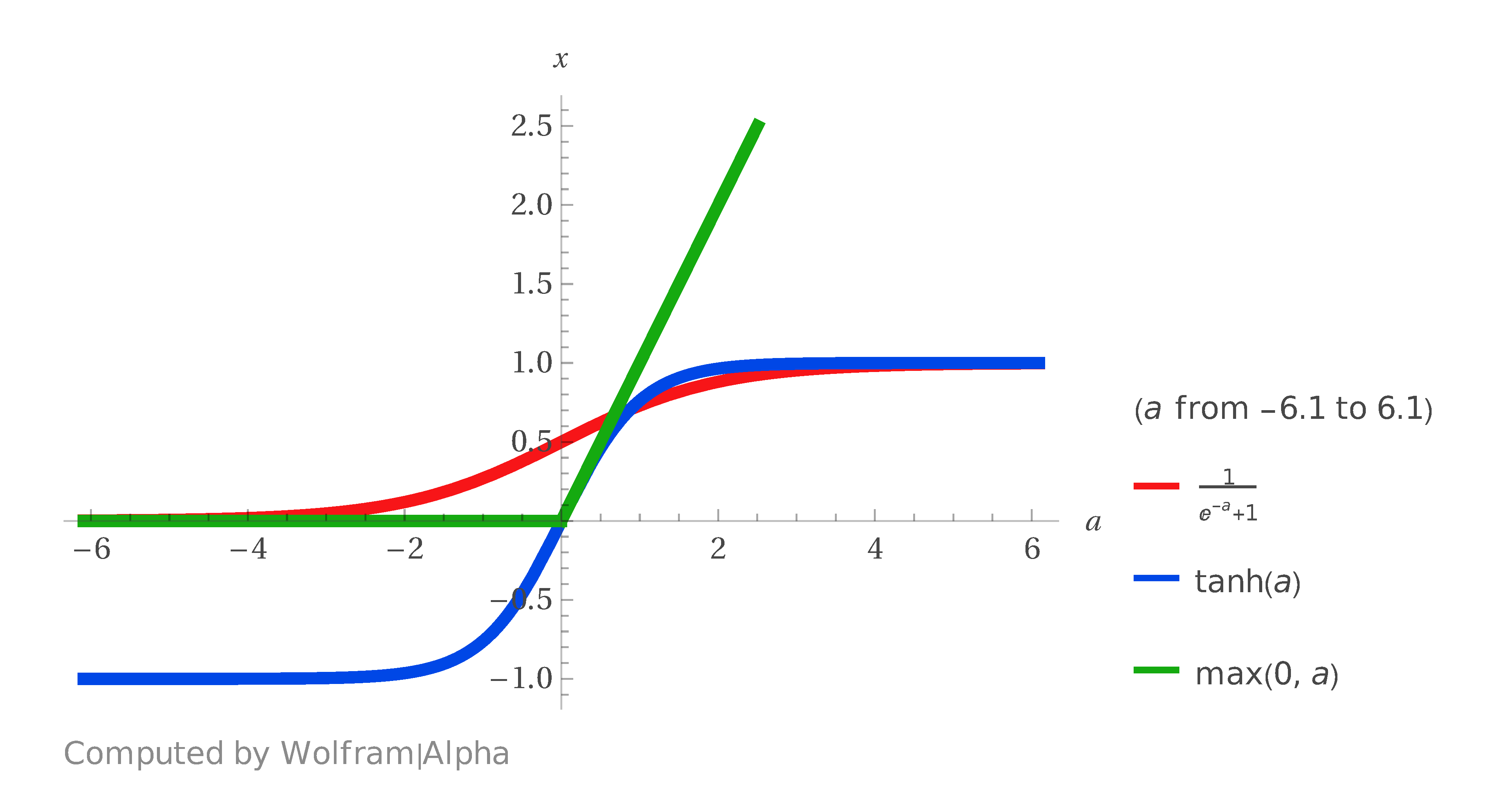
The hyperbolic tangent function is a mirror transformation of the sigmoid via $$\tanh(a)=2\times\operatorname{Sigmoid}(2a)-1,$$ so that it is centered around zero, that is, $\tanh(0)=0.$

Hence, we can show that the hyperbolic tangent function generates the same class of networks as the sigmoid function subject to some linear transformation of weights, meaning that they are equivalent when making forecasts.